PhotoChrome 6.44

User Guide

QuickStart: Setup / Usage

PCS is a Posix application. This means it is written primarily for a *nix (Linux, Mac) environment but it also operates in a Windows environment (via MinGW – providing Posix compatibility on Windows).

Windows note: Earlier versions of PCS for Windows distributed Cygwin binaries and required matching shared DLLs. New versions use MinGW instead which requires just the .exe. Less fuss!

There are no other prerequisites for using the tool. It operates from the command line.

If you are using a different kind of operating system the tool can be compiled from source. The image libraries needed for Windows, Linux and Mac builds are included with the source.

Basic usage pattern...

From DOS prompt:

   pcs [options] [-o outfile.pcs] infile(s) 

Or from a Linux/Mac shell:

   ./pcs [options] [-o outfile.pcs] infile(s) 

The output file will default to INFILE.PCS but can be overloaded with ‘-o’.

Input images can be .png, .jpg, .tga or .bmp. The output name is the input name with its extension replaced by .PCS, for every storage format.

If you specify infile as a GLOB for batching (e.g. *.PNG) overloading should be avoided – each output file will be named according to the corresponding input file. -o with more than one input file is an error.

Don’t enable diagnostic mode when batching multiple PhotoChrome conversions in one job – the diagnostic files are written to the current folder and will be overwritten for each image. CryptoChrome modes file each source's outputs in its own folder when given several sources (see -ccmode).

QuickStart: Test - STE Output

For quick results on an STE from a 29,791 colour palette & no dithering - try one of the sampling reduction methods e.g. -m 4:

   pcs -cd ste -f 2 -m 4 -lt 3 -dt 0 -et 0 test.jpg

If you don’t mind waiting and want to concentrate on image quality, or if the image is causing difficulties with high colour variation, try the neural network colour reducer in dual-field mode at a refinement depth of 12 (4096 iterations) with 4 passes of field error diffusion.... And make a cup of tea or go for a walk.

   pcs -cd ste -f 2 -m 5 -nnd 12 -lt 3 -dt 0 -et 1 -ei 4 test.png

Some less challenging images can look more accurate and stable (and produce smaller files) using only palette interlacing (‘shared bitmap’ mode). Sometimes it’s worth trying this because when it works it can produce the most stable display. Files are smaller because only one bitmap needs to be displayed, and both palette fields are very similar. This mode is not as powerful as dual-field mode for dealing with colour variation and shading – look out for visible streaks and patches.

   pcs -cd ste -f 1 -fm 1 -m 5 -lt 3 -dt 0 -et 2 test.png

And for 100% stability (but without the extended palette – 4096 colours only), you can use this to generate a single-field image with error-diffusion added:

   pcs -cd ste -f 1 -m 5 -dt 0 -et 2 test.png

QuickStart: Test - ST(FM) Output

The ST(FM) equivalents for the above cases is the same – just pass ‘-cd st’ instead of ‘-cd ste’ to generate the appropriate colour depth.

Due to the reduced colour depth, some settings will be more or less appropriate for ST vs STE.

E.G. some types of dithering look better at higher colour depths while others suit lower colour depths. These are all explained later.

Command Reference: Basic Controls

-?
-h
--help

Print usage information to console.

-v
--verbose

Print more verbose messages during conversion.

-q
--quiet

Suppress/minimize messages not essential for status (e.g. for batching).

-k
--wait-key

Wait for a keypress after conversion (typically for testing scripts only).

-dump
--dump

Print the current value of every setting, then exit. Switches given before -dump are reflected in the output; anything after it is not read.

-ek
--err-wait-key

Wait for a keypress when conversion stops on an error. Errors in the switches themselves exit without waiting.

Command Reference: Diagnostics

-dg
--diagnostics

default = disabled

Emit diagnostic information and images relating to conversion process. This helps judge quality and success, and the impact of changing settings related to conversion.

Diagnostic message log:

> converting image...
iteration: 200/ 256, radius(0.201), alpha(0.000387), sqerr:79.19   ← A
iteration: 200/ 256, radius(0.201), alpha(0.000387), sqerr:79.02
performing diagnostic passes...
Bias = 1.022746 / 255 (0.4011%)   ← B
uRange = -0.222088 / 255 (-0.0871%) ← C
lRange = -0.314308 / 255 (-0.1233%)
nRange = 0.706596
LinERR(virt) = 1.631126%  ← D
VecERR(virt) = 3.840731%
SquERR(virt) = 0.00014040
LinERR(8bit) = 1.981791%
VecERR(8bit) = 4.058464%
SquERR(8bit) = 0.00013958
writing field 0 diagnostic...
writing field 1 diagnostic...
writing final diagnostic...
> creating output file…

A: Some algorithms will print an error metric during reduction to show progress towards error convergence. Generally if shown, it should reduce. If it seems not to reduce, or coasts on without reducing after some time, the settings probably could do with adjustment.

B: Bias = normally be close to 0.0% for a well-centred image. Values far from zero will suggest that the image is either brighter or darker than the original, because the colours involved rounded towards displayable colour depth, and more rounded in one direction (+ve) than the other (-ve). The figure is shown in % and in terms of E/255 to where E is a single grey level in 24bit space.

C: uRange = mean error for upper half of intensity range. lRange = mean error for lower half of intensity range. nRange = ratio of one to the other. If nRange is not close to 1.0, it means error is concentrated on either brighter or darker colours. Used to debug conversion of grey-level testcards where these figures are predictable for known images.

D: LinERR/VecERR/SquERR are numerical estimates of error for the final image.

LinERR = linear error (normalized)

e = (sum((eR/3)+(eG/3)+(eB/3)) / pixels) * 100%

Practically a (normalized) subtraction of the source and final images.

VecERR = vector distance error (normalized) 

e = (sum(sqrt(sqr(eR)+sqr(eG)+sqr(eB))) / pixels) * 100%

The represents a (normalized) linear sum of individual pixel vector errors.

SquERR = RMS (root mean square) error

e = sqrt(sum(sqr(eR)+sqr(eG)+sqr(eB)) / pixels)

This is the RMS (root mean square) of the per-pixel colour error vector for the image.

As with the diagnostic images below, error is calculated in both 8bit (24bit source image) space and in virtual display colour space.

LinERR(8bit) = source colour space (includes colour depth losses)
LinERR(virt) = virtual display space (excludes colourdepth loss)

The ‘virt’ metrics are more representative of error when comparing between different algorithms during colour reduction - but it is somewhat irregular/imprecise because there are ‘steps’ in this colour space so an increase in reported error doesn’t necessarily mean the conversion got worse.

It is therefore recommended to optimize images using the SquERR(8bit) metric as the primary guide.

Diagnostic images generated:

srcref.png 

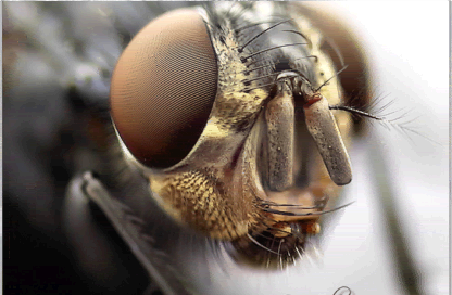
This is the reference source image after resizing/preprocessing, but before colour reduction. It can be directly compared with the preview.png image. Any differences between the input image and srcref.png are likely due to auto resizing and should be discounted when checking conversion results.

preview.png

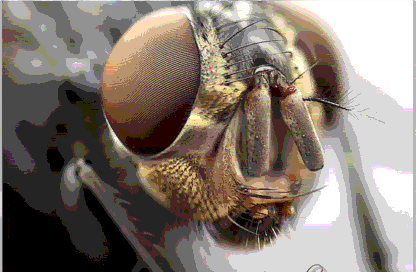
Final image preview, combining all fields in their native colour depths into the ‘virtual’ colour depth to be experienced on the display. Flicker of course is absent!

field?.png <0-N>

Final field preview, for field N of a multi-field image. Only written for multi-field images.

Walking through field previews in a PNG viewer helps estimate flicker or shimmer patterns, albeit more exaggerated than the real display. Note that individual fields can look odd due to lace settings, and particularly if error-distribution mode 1 is used to bounce error between fields.

bias.png

This image maps the error area bias between the srcref and final images. The area bias should ideally be balanced (-ve errors compensate for +ve errors elsewhere). This rarely happens because the error magnitude varies across the image and colour reduction chases a minimum squared error sum.

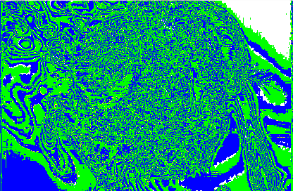
Green indicates +ve error while blue indicates -ve error. White indicates exact match, yellow means < epsilon error (near enough a match - some CR algorithms don’t deal in exact colours).

The error being represented includes (and is largely made up of) source colours which can’t be represented in the native colour depth. This results in characteristic blue/green alternation.

The bias preview is partly a colour reduction debugging tool (to check that range is centred and fully used) and partly for highlighting the difference between poor colour reduction (horizontal streak glitches) and poor colour depth representation on the final display device (which appears as nice alternating blue/green contours).

linerr8b.png
linerrnv.png

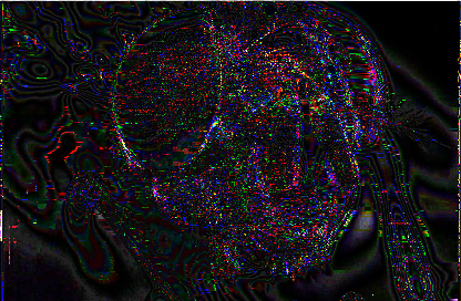
These images encode the linear (RGB) colour error between the srcref and final images. With the perception filter mask working effectively, this error will end up concentrated on and around edges, avoiding smooth areas. Since linear error difference tends to be small, these images will probably need contrasted up to see anything meaningful.

The ‘8b’ postfix indicates error in 8-bit colour space (really, 24bit RGB). i.e. literal difference between the srcref.png image and the preview.png image. It therefore includes error relating to un-achievable colours on the native display - error that the algorithms can never remove. This can be a bit misleading if the aim is to compare algorithms...

The ‘nv’ (native virtual) postfix indicates error in ‘virtual’ colour space. This is a more honest estimate of colour reduction algorithm success because it excludes colours which can never be shown on the native display.

e.g. for an STE image in 2-field mode, only 31 grey levels are possible, (versus 256 in the srcref). The error information encoded in linerrnv.png will therefore only contain deviations between the final image and a 31-grey level version of srcref.png. In other words - any errors encoded here are related to the colour reduction step alone, and not limitations of the native display.

vecerr8b.png
vecerrnv.png

These images encode the vector (squared) colour error between the srcref and final images. This is how the colour reducer sees error and attempts to minimize it within the image. Larger error spikes with a small area are punished more severely than small errors over a large area - edges appear exaggerated in these previews in the same way the algorithm sees them. The perception filter mask provides some control over this.

These are usually fairly easy to view directly, without needing any additional manipulation.

Tip: The easiest / most interesting image to view for estimating general success at colour reduction (or comparing the algorithms) is the vecerrnv.png diagnostic.

pcfmask.png

(See also -pfmi, -pfmg, -pfms)

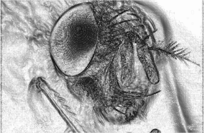
This is a visualization of the perception filter mask, which guides colour error tolerance while choosing colours. Darker areas represent edges and will tolerate more error. Light areas represent fine shading / flat colour and get extra care from the colour reduction algorithms.

Command Reference: Storage/Export Formats

-s         <formatcode>
--storage  <formatcode>

default = 0 (PPRLE)

(See also section on custom conversion profiles)

Specify output file format. This is useful mainly when generating images using custom timing patterns. Adopting the simplest possible format can help debug image display code. By default the original PCS v3,v4 format is used, which includes a header and some weak compression of bitmap/palette data.

Some combinations change the format: a custom -pct selects format 2 in place of 0, 1 or 4, and 3- or 4-field images (-f 3/4) are written as format 1 in place of 0. Format 4 is accepted but writes no image data.

0 – PPRLE:                 plane-by-plane RLE with header (v3,v4 compatible)
1 – UNCOMPRESSED:          as #0, without compression (v3,v4 compatible)
2 – DIRECT_DISPLAY:        raw display format, retaining PCS header
3 – RAW_DISPLAY:           raw bitmap+palette display format, minus PCS header
4 – COMPRESSIBLE:          chunky nibble format for LZ? - not implemented
5 – RAW_ILEAVED_DISPLAY:   as #3 with 2 fields interleaved into one frame

Formats 3 (RAW_DISPLAY) or 5 are probably the easiest to test/debug when implementing a new timing pattern since the bitmap and palette data are raw, separated and no header is present.

Format 5 is for 2-field images on an interlaced display: field 0 provides the even lines and field 1 the odd lines of a single frame (bitmap, then palette). With other field counts it is the same as format 3.

Command Reference: Image Conversion

-f         <num>
--fields   <num>

default = 2

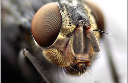
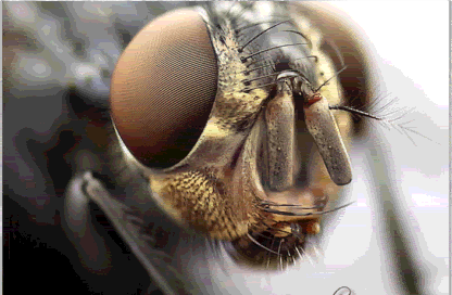
Number of fields to generate for display. More fields means more colours (and more memory, bigger files). Below: single-field image (left) compared with a tri-field image (right).

PhotoChrome versions v5.x and below could generate single-field or dual-field images in 3 different field modes. The multi-field images depend on bitmap and/or palette flipping at 50/60Hz to display correctly.

PhotoChrome v6.x can now generate tri-field and quad-field images, producing many more colour shades. These work in exactly the same way, requiring only minor changes to loading/display code. Such images are however more complex to generate and there are additional controls available to optimize flicker & interlacing patterns for these. It may take some time and experimentation to settle on the best options for any given image.

-wp
--wake-prot

default = disabled

ST/STE machines can exhibit a strange electronic timing effect which causes palette-blasting display routines to occur 1 pixel out of sync with the image bitmap. This often causes columns of dots to appear on hi-colour images, which may go away (or reappear) if the machine is power-cycled. It is a well known issue and affects all types of hi-colour display routine in low resolution (However, note that it may not affect medium resolution at all).

Enabling this switch will encode the image with a ‘wakeup protection’ technique and this will effectively immunise the image against the dreaded dots. There is a tiny loss in available colour count as a result, which may affect conversion quality of very tough images - but it’s almost always worth using because the image will look far worse if the dots appear on the viewer’s machine...

-wp is kept so that existing command scripts still work, but it rarely changes anything: the builtin profile always applies wakeup protection (through its builtin DPT), and -wp is ignored when a -dpt table is given. It only takes effect with a custom -pct and no -dpt.

-fm        <mode>
--fieldmode     <mode>

default = 0 (NOSHARING)

When generating multi-field images, a field mode may be specified which controls which components will require strobing/cycling during display.

Shared-bitmap mode (1) needs -f 1; shared-palette mode (2) needs -f 2 or more.

The 3 field modes are:

0 - NOSHARING:      N bitmaps + N palettes (normal multi-field image)
1 - SHAREDBITMAP:   1 bitmap + N palettes
2 - SHAREDPALETE:   N bitmaps + 1 palette

Caution: Pay attention to the section on file formats since data is not necessarily stored in the order suggested above, especially for shared- component images, where cloned data may be exported for shared fields.

Shared-bitmap mode:

This mode generates one bitmap and 2 palette fields. It is chosen by specifying -f 1 -fm 1 (yes... single field mode!). It operates internally as if processing a single field but with a higher bitdepth palette, and splits the palette in two during the final stages of conversion.

In terms of data written out (storage mode 3) it will appear as a normal two-field image with two bitmaps. The extra bitmap just happens to be duplicated - it can be ignored.

For streaming hi-colour video, it can be beneficial to use shared-bitmap mode because then it is only necessary to store one bitmap for each two 50Hz fields displayed. The bitmap can be updated at 25Hz, while the palette can be updated at 50Hz. The 50Hz palette pairs will also delta-compress well because they both correspond to the same bitmap (i.e. they will be stable with respect to one another, unlike multi-bitmap images), with only in-between shades encoding deltas for the 2nd field.

Shared-palette mode:

Implements the opposite - a fixed palette with multiple bitmaps. Either sharing mode may be useful at reducing the storage cost of 3- and 4-field images, with different visual compromises. It may find additional uses but the other modes are more versatile.

-pl
--prelace

Treat the source as pre-interlaced, requiring de-interlacing to dual-fields: requires -f 2. The source is sized to twice the output height; field 0 takes the even source lines and field 1 the odd lines (e.g. a 320x400 source for a 320x200 two-field image). A mask given with -pfms must also be twice the height. PhotoChrome mode only.

-cd             <bits>
--colour-depth  <bits>

default = STE

Colour depth specifies which machine the image is targeting - ST or STE. For PhotoChrome images there are only two settings which currently make sense. Higher depths are used only by CryptoChrome palettes made with -ccmethod sopn (e.g. for Falcon030).

3    ST    (9bit, or 512 native colours)
4    STE   (12bit, or 4096 native colours)
6    F030  (18bit, -ccmethod sopn only)

Note that the colour depth specifies the native bitdepth of the hardware. It is not the bitdepth of the perceived image. The number of fields generated will affect the perceived bitdepth. e.g. for ST/STE the colour counts are:

Below: STE single-field image on the left compared with ST single-field image on the right. No dithering used, to highlight the difference.

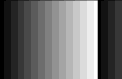
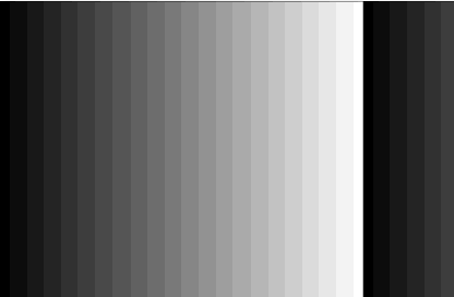
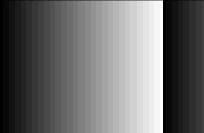
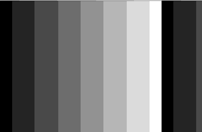
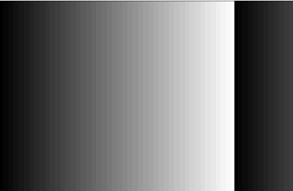
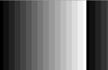
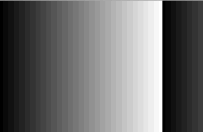
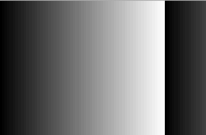
Below: Greyscale testcards for all 8 'native virtual' colour depths. (Top row: ST Bottom row: STE)

-pc             <2-8>
--plane-count   <2-8>

default = 4

Number of bitplanes, giving 2^planes colours per palette. For PhotoChrome, a custom PCT sets this itself (see -pct). For CryptoChrome: -ccmethod de needs 4, -ccmode 1 (Degas) allows at most 4, -ccmethod sopn allows 2-8 (up to 256 colours). With -ccmode 7 (ApplyPalette) it can be left out; if given it must match the palette.

-m
--method

default = 4

The conversion method specifies the algorithm used to convert the image from 24bit colour down to the complementary field & palette data for native display. Since this conversion is a global optimization problem with many solutions, a choice of algorithms is provided to experiment with. Each has some benefit (e.g. speed, memory consumption, quality, consistency, sampling vs analytical...)

The methods (or algorithms) are listed here:

0    SIMPLE           Sample lines left->right, top->bottom.

This is the simplest, quickest method but the results are usually very poor because leftmost pixels get priority, having been processed first. Later pixels are forced to use colours already chosen by earlier ones. Mainly included for comparison & debugging.

This is a sampling algorithm. It uses real source colours so if there is no colour competition in the image, it will be 1:1.

1    SUBDIVISION 1    Sample lines in subdivision pattern, row order.

As fast as method 0, but colour allocation is more fair within a line. Scanlines subdivided until colours exhausted. lines are processed one at a time. However the quality is still inferior to other methods. The primary benefits are speed and low memory usage. It is similar to the algorithm used in the original PhotoChrome v3, v4 for ST but slightly improved.

This is a sampling algorithm. It uses real source colours so if there is no colour competition in the image, it will be 1:1.

Can induce streaking because lines are solved in top-to-bottom order, forcing lines to use some colours already claimed by the line above, without guiding the production of those colours. This is a classic ordering problem encountered with any sampling-based solver. The different sampling algorithms just hide the ordering problems in different ways...

2    LCG              Linear Congruential Generator (pseudorandom sampling)

This is another form of subdivision sampler, operating instead on the whole display. It efficiently samples all pixels in pseudorandom order until all have been processed. This is also fast and uses little memory - but results can differ from method 1.

While better than method 1 in general, it can induce random localised streaking because it is still a sampling solver which causes some pixels to be treated more fairly than others (i.e. the pixels getting processed first get the most accurate colours).

This is a sampling algorithm. It uses real source colours so if there is no colour competition in the image, it will be 1:1.

3    BIN BALANCE L    Global solver type 1: fast, low quality

The bin-balancer is a custom algorithm made for PhotoChrome. It is a global solver so it operates on the whole image at once. It does not suffer from ordering problems seen with the sampling methods. It is good at dealing with display timing patterns which share palettes across the left/right border.

It does however consume a lot of RAM, like the other global solvers, and is relatively slow to compute. While results are generally good, there are 2 other solvers which almost always produce better results.

For converting video or very large batches of images, this is a decent choice vs conversion speed. Method 5 can be configured to convert more quickly if needed, but not necessarily with better (or equal) results. Method 3 is kept for this reason.

This is an analytical algorithm. Colours are generated to satisfy sharing between pixels which want slightly different colours. It is therefore potentially lossy. However lossyness for this algorithm is proportional to image complexity - it can be minimal or zero for trivial inputs.

4    SUBDIVISION 2

This is the same as method 1, but attempts to suppress streaking by processing pixels in column-order instead of row-order. The display is subdivided a column at a time, with a whole column being processed at once. This treats lines more fairly, at the expense of horizontal neighbours.

Generally though, it is better to use one of the global solvers for most images.

5    SOM              Self Organizing Map / Neural Network solver

(see also: -nnd, -nnb, -nnr)

This is by far the most powerful and flexible algorithm. It was developed specially for PhotoChrome, based loosely on a known effective algorithm for generating palettes (NeuQuant). There are a number of important differences in the PhotoChrome SOM algorithm - not least it’s ability to solve multiple constraints at once (huge number of connected palettes with overlaps). It also incorporates some neural network learning accelerators (training momentum, managed convergence being two).

The SOM algorithm generally yields the best results in the majority of cases. There may be exceptions, and for specific scenarios there may still be value in using the others (e.g. converting long video sequences might benefit from the speed vs quality of method 3, or a lower-quality sampling method, especially for preview/trial conversion jobs). However if needed, at the expense of quality, this method can also be configured to run very quickly by reducing iterations.

There are a number of tweak factors affecting this algorithm, but the most useful is probably ‘-nnd’. This allows the convergence depth (number of solver iterations) to be specified. The more iterations, the better the result - up to a point. Too many iterations can begin to go in the other direction. The optimal setting tends to lie between 8 and 10 for most cases. Lower values for previewing batch jobs only.

This is an analytical algorithm. Colours are generated to satisfy sharing between pixels which want slightly different colours. It is therefore lossy. It excels for complex input, but can produce weird results for trivial input (e.g. a grayscale testcard can produce grey bands of different widths) because it is numerical, statistical and doesn’t guarantee settling on original colours.

6    BIN BALANCE H    Global Solver type 2: slow/high quality

This is almost exactly the same as method 3, but includes an extra reduction phase which improves colour selection, at the price of taking much longer. It is the slowest algorithm in the set.

Often results will look similar to method 5, but in most cases method 5 will yield equivalent results in less time, or better results in similar time. However there may be rare cases where this wins. It’s kept for that purpose.

This is an analytical algorithm. Colours are generated to satisfy sharing between pixels which want slightly different colours. It is therefore potentially lossy. However lossyness for this algorithm is proportional to image complexity - it can be minimal or zero for trivial inputs.

-lt             <type>
--lace-type           <type>

default = 3 (CHECKER)

(see also: -mladj, -ls)

This control is only meaningful for multi-field images. (i.e. -f >= 2)

Multi-field images are strobed (or cycled, if more than 2) and this strobing would normally cause obvious flicker - the average brightness of one image will be higher than the other. New shades are generated by averaging two images with a brightness offset of 0.5 native colour bits (or -0.25 / +0.25).

field 0:        field 1:
0 0             1 1
0 0             1 1

To control this flicker, the ideal solution is to interleave / interlace the two fields together, such that both fields combine half of the information from each image. Each field now has the same average brightness, and strobing them doesn’t present obvious flicker.

Field 0:        field 1:
1 0             0 1 
0 1             1 0

If there were no other issues with this, it would be enough to have a single interlacing pattern. Unfortunately there are several issues with it.

The biggest problem is colour starvation. Stippling can as much as double the number of shades required to render a group of pixels within a single colour change event (a short horizontal span of pixels). If colours are muted it can work well, but under pressure with a lot of different colours it causes horizontal streaks.

A second issue relates to multi-field images with more than 2 fields. For a 3-field image, the offsets are -0.3, 0.0, +0.3. There is more than one way to stipple 3 different values in 3 dimensions (x,y,f). It’s even more complicated with 4 fields.

To help deal with this, several interlacing patterns are supported, each with different strengths.

0 - FIELD

No interlacing. Fields are left separate.

0 0             1 1
0 0             1 1

1 - HORIZONTAL 

Fields are interlaced as complete scanlines. This results in efficient colour use and is effective at reducing flicker. It may however compete with scanline display on CRTs.

0 0             0 0
1 1             1 1

2 - VERTICAL

Fields are interlaced as columns. This won’t normally produce less streaking than CHECKER but can if conversion method 4 (-m 4) is in use, which processes pixels in column order.

0 1             0 1
0 1             0 1

3 - CHECKER

Fields are interlaced with a checker pattern.

1 0             0 1 
0 1             1 0

4 - PRNG

Pseudo-random number generator. Fields are interlaced with random distribution. This produces reasonably good results but more visible than CHECKER and still can cause streaks.

1 1 0 1         0 0 1 0
0 1 0 0         1 0 1 1
1 0 1 0         0 1 0 1

5 - OFF

No interlace offsets at all. This is selected automatically for single-field images (-f 1).

-mladj     <0-6>
--mlace-adj     <0-6>

default = 0

For 3- and 4-field images, there are many different ways to cycle through the interlace offsets because it is not a simple strobe but a carefully ordered number sequence. The sequence must be distributed in time-and-space to prevent a single field from appearing either brighter than the others, or containing visible patterns.

This switch provides a choice from one of several different variants on each of the interlacing types specified with -lt. Some types do not provide variants (and none provide extra variants with 1 or 2 fields).

A variant which doesn't exist for the lace type and field count falls back to variant 0.

Note: ‘countercycling’ means adjacent pixels (on at least one axis) cycle through the 3 (or 4) interlace offsets patterns in different directions. The patterns being cycled through are not necessarily ordered (e.g. 1,3,0,2) and the sequence may also be different for adjacent pixels. The combined effects are sometimes but not always beneficial. Experiment!

tri-field images (-f 3):

FIELD:
HORIZONTAL:
VERTICAL:
(no variants)

CHECKER:
0      cycling 3x3 checker tile
1      Y-axis countercycling 3x3 tile
2      2D countercycling 3x3 tile
3      cycling 4x4 checker tile
4      Y-axis countercycling 4x4 tile
5      2D countercycling 4x4 tile
6      X-axis countercycling of reordered rows

PRNG:
0      cycling pseudorandom distribution
1      pseudorandom countercycling distribution 

quad-field images (-f 4):

FIELD
(no variants)

HORIZONTAL
0      ordered rows
1      unordered rows

VERTICAL
0      ordered columns
1      unordered columns

CHECKER:
0      cycling 4x4 checker tile
1      Y-axis countercycling 4x4 tile
2      2D countercycling 4x4 tile

PRNG:
0      pseudorandom cycling distribution

1      pseudorandom countercycling distribution 

-ls
--lace-sync

default = disabled

In a final bid to optimize colour allocation, flicker and streaks, this method has been introduced as an adjustment to the patterned -lt lace types which toggle the horizontal axis (VERTICAL, CHECKER). It does not apply to PRNG, which would no longer be random and would show visible patterns.

Instead of toggling every pixel (or multiples of a pixel) the lace-sync mode puts the horizontal axis into the same space as the palette change timing. This means the interlace offsets are constant within a colour change timing slot - which usually lasts a few pixels. This is theoretically optimal. However using CHECKER on its own is still visually better if the image isn’t struggling with colours so this is really a last resort. It seems most useful for the 3- and 4-field images.

Note that this acts as a modifier on top of the existing -lt setting. It really just stretches the pattern horizontally to match the timing pattern.

CHECKER:

1 0                   0 1 
0 1                   1 0

..becomes

11111111 00000000          00000000 11111111 
00000000 11111111          11111111 00000000

-dt             <type>
--dither-type   <type>

default = 0

To fill in for colours in the source image which can’t be generated with the chosen number of fields, the offset-dithering system can be useful. Several dither patterns are available to choose from and the dither strength can be adjusted. It is called offset-dithering because it selectively offsets the brightness of pixels in a specific pattern. Typically the offset is a fraction of a display ‘colour bit’ i.e. less than a single grey level on the display.

0 - NONE

No dithering.

0, 0
0, 0

1 - PRNG

Pseudo-random grey level distribution.

2 - STIPPLE

Standard 2x2 dither pattern. This simulates an extra shading ‘band’ between two native colours. Sometimes this is still visible so other patterns are generally better.

0, 1
1, 0

3 – CPRNG

Pseudo-random RGB distribution. This theoretically produces more shades, better dithering than PRNG, but it significantly increases colour allocation pressure. Will only work well with specific images.

4 - TINY (3x3 matrix dither)

2, 6, 4
5, 0, 1
8, 3, 7

5 - BAYER 4 (4x4 matrix dither)

 0,  8,  2, 10
12,  4, 14,  6
 3, 11,  1,  9
15,  7, 13,  5

6 - MESHED (4x4 matrix dither)

11,  4,  6,  9
12,  0,  2, 14
 7,  8, 10,  5
 3, 15, 13,  1

7 - PAN MAGIC (4x4 matrix dither)

 7, 10, 13,  0
12,  1,  6, 11
 2, 15,  8,  5

 9,  4,  3, 14

8 - BAYER 8 (8x8 matrix dither)

 1, 33,  9, 41,  3, 35, 11, 43
49, 17, 57, 25, 51, 19, 59, 27
13, 45,  5, 37, 15, 47,  7, 39
61, 29, 53, 21, 63, 31, 55, 23
 4, 36, 12, 44,  2, 34, 10, 42
52, 20, 60, 28, 50, 18, 58, 26
16, 48,  8, 40, 14, 46,  6, 38

64, 32, 56, 24, 62, 30, 54, 22

-dl             <-8.0-8.0>
--dither-level  <-8.0-8.0>

default = 1.0

Normally dithering is performed at full strength (1.0) but it may be toned down using this option. A value of 0 is equivalent to turning it off. It can also be exaggerated using values > 1.0. Exaggerating causes dither bands to overlap. Reducing creates gaps between dither bands.

-et             <type>
--error-type    <type>

default = 0 (NONE)

(see also: -ei, -el, -spet)

There are several ways to deal with colour allocation error in generated images. Colour allocation error combines both failures to find a good colour (due to exhausting the palettes) and inability to represent colours outside of the shading range for the output image type. Any deviation of final pixel colour from the original reference image is measured as colour error and this can be used.

For single-field images, either the error is accepted as-is, or it can be re-distributed around the image. Floyd-Steinberg is an example of a 2D error-distribution algorithm and it appears as another type of dithering (despite having a completely different effect from offset dithering). This approach is called SPATIAL error feedback because the error is fed back into the image at different location.

For multi-field images a more sophisticated trick can be used to improve the final image. Instead of distributing error around neighbour pixels, the error can be ‘pushed’ into one of the other fields where it gets a chance to be absorbed (really, compensated for). The colour error can be bounced back and forth over several iterations until all fields absorb part of the error. This is called FIELD error feedback.

0 - NONE
1 - FIELD FEEDBACK
2 - SPATIAL FEEDBACK

Note 1: For FIELD mode, the number of iterations must be specified separately (-ei). For SPATIAL mode, the algorithm (dither pattern) can be specified separately (-spet). For both modes, the error level (strength) can be set separately (-el).

Note 2: It doesn’t really make sense to use offset-dithering with SPATIAL error distribution - they will compete and it will look ugly.

Caution: Because of the way SPATIAL error distribution works, it has to use available colours to dither with. It does not itself guide the creation of new colours because it can’t predict what errors will occur before the palette is generated. This can lead to some nasty side effects in rare cases where enough shading error collects in an area of the image but can’t be dithered out in a suitable colour. Normally this won’t happen in normal images because there’s one palette for all pixels. But in PCS images there lots of local palettes and some will contain a very narrow set of shades, which don’t error-distribute well. Worse, the success varies from palette to palette, across the display.

What happens is this: The error builds up from the dominant shades, unaddressed until almost any colour will do as a dither - and you get a bright speck appearing (or a thinly distributed cloud of them). What it is doing here is technically correct - but it’s working with a very limited set of locally available colours. This tends to happen if the image has lots of shades of the same colours, but a small number of very different ones (like a large selection of dark greens, plus one yellow) - the inappropriate colour(s) eventually get employed to dither the accumulated error from use of the other more dominant shades. If a lighter green had been available in the palette at that location it would have been used instead and more frequently. Instead yellow specks are used, widely spaced, because that’s all it has to work with for those pixels.

I might be able to fix this in future by limiting the maximum error which can accumulate, or by punishing choices with a large error distance for a single pixel - but for now just try different settings or abandon -et 2 completely for affected images. It works well however for images which have a good spread of colours in most parts of the image.

-el             <0-100>
--error-level   <0-100>

default = 99.9

When using -et to specify an error distribution method, this can be used to adjust the strength of the feedback (percentage of feedback). It is particularly important for FIELD mode, since the system works best if only a portion of the error is pushed between fields. Pushing the full error can cause the fields to diverge and produce visible artifacts.

e.g. for 80% field-feedback on a 2-field image with 3 error iterations:

-f 2 -et 1 -ei 3 -el 80.0

-ei             <2-49>
--error-iters   <2-49>

default = 2 with -et 1 (otherwise unused)

Specifies the number of times to bounce colour reduction error between fields in a multi-field image (FIELD feedback, -et 1). The first pass is uncompensated, so at least 2 are needed for any effect; if -et 1 is given with a lower -ei, 2 is used. -ei has no effect without -et 1. A good value is 3, but it needs experimentation for each image.

-spet           <type>
--spatialerr-type     <type>

default = 5 (STUCKI)

Specify the SPATIAL error distribution algorithm (-et 2). There are lots of these so it’s worth looking up more detail on the pros/cons of each if you plan to use them.

0 - FLOYD-STEINBERG
1 - JAJUNI
2 - ZHIGANG
3 - SHIAU1
4 - SHIAU2
5 - STUCKI
6 - BURKES
7 - SIERRA
8 - ATKINSON

-nnd       <1-20>
--nn-depth <1-20>

default = 10

This adjusts the performance of the Self-Organizing-Map (SOM) colour reduction algorithm available in various modes/stages. It specifies the number of convergence iterations performed by that algorithm. Good values are usually between 8 (fast) and 10 (slow) with higher values generally giving better results. Sometimes the opposite is true so it’s worth using the diagnostic figures to monitor error level and find the best setting that way. e.g.

-m 5 -nnd 9

Note: Used by conversion method 5 (SOM) and by CryptoChrome -ccmethod sopn. Not used by any other method.

-nnb            <0.01-1.0>
--nn-breadth    <0.01-1.0>

default = 0.1

This adjusts the performance of the Self-Organizing-Map (SOM) colour reduction algorithm available in various modes/stages. It specifies the proportion of the training samples re-presented on each cycle. Higher values give fresher neighbourhoods on each cycle, but take longer.

Too small a setting will prevent the algorithm from converging properly. Too large a setting will perform poorly in other ways, differentiating related colours less effectively (and also take longer). In general it’s not necessary to adjust this but it can be tweaked +/- for specific images if a benefit can be measured in the diagnostic report. e.g.

-m 5 -nnd 9 -nnb 0.2

Note: Used by conversion method 5 (SOM) and by CryptoChrome -ccmethod sopn. Not used by any other method.

-nnr       <>0.0-1.0>
--nn-rate  <>0.0-1.0>

default = 0.0025

This adjusts the performance of the Self-Organizing-Map (SOM) colour reduction algorithm available in various modes/stages. It specifies the rate of convergence on each iteration. Generally with more iterations, it is better to reduce the convergence rate so the algorithm doesn’t overshoot.

Normally this setting can be left alone, but with -nnd >= 10, it may need to be adjusted lower for best results. e.g.

-m 5 -nnd 11 -nnr 0.001

Note: Used by conversion method 5 (SOM) and by CryptoChrome -ccmethod sopn. Not used by any other method.

-nnrad           <>0.0-256.0>
--nn-radius      <>0.0-256.0>

default = 10.0

Starting neighbourhood radius: how far along the network each training step reaches, shrinking as training proceeds. The tool prints a suggested ballpark for the image.

-nnm             <>0.0 to <1.0>
--nn-moment      <>0.0 to <1.0>

default = 0.95

Learning momentum: neurons keep part of their previous movement on each update, which speeds convergence. Lower values damp it.

-nnrho           <>0.0 to <100.0>
--nn-rho         <>0.0 to <100.0>

default = 4.0

Grouping gradient: how sharply influence falls off with distance inside the neighbourhood radius. Higher values keep training more local.

-nnt             <strip,ring,grid,tiled>
--nn-topo        <strip,ring,grid,tiled>

default = ring

Network topology, i.e. which neurons count as neighbours:

Method 5 needs at least 4 colours for grid/tiled. With -ccmethod sopn and -ccfields 2 the network is made of colour pairs rather than colours.

Note: Used by conversion method 5 (SOM) and by CryptoChrome -ccmethod sopn. Not used by any other method.

-pfmi           <0.0-1.0>
--pfm-influence <0.0-1.0>

default = 0.99999

(see also: -pfmg, -pfms)

The conversion algorithms will try to use a perception-oriented view of acceptable error in colour choices. It will try to reduce error in areas which are more likely to be noticed, trading for additional errors in places where they are less visible. This has to do with the separation of colour and intensity sensitivity in the eye, and edge detection sensitivity of the eye.

Generally the eye will notice glitches in finely shaded areas or smooth areas, but will have difficulty picking up glitches on or near edges. The PFM (peception filter mask) is an image mask artificially generated by the tool, which guides error reduction for the image.

With diagnostics enabled (-dg) the PFM will be emitted as a pcfmask.png file. Interpreting this mask is easy - lighter areas will receive more attention for error correction, whereas dark areas will be less sensitive to error correction. Edges in this image will therefore appear dark.

Reducing -pfmi will reduce the influence of the mask, and therefore increase the brightness/reduce the contrast of the mask, approaching white at -pfmi=0. This effectively turns off the PFM.

-pfmg      <0.0-100.0>
--pfm-gamma     <0.0-100.0>

default = 1.0

(see also: -pfmi)

This allows the gamma curve for the PFM to be adjusted, which may help tune conversion of some images, especially when combined with -pfmi. It takes time to experiment with these options. -pfmg 2.0 will sharply increase the contrast of the mask. -pfmg 0.5 will reduce it. Monitor the pcfmask.png diagnostic image to make sure it doesn’t get too dark, indistinct or too light.

-pfms           <maskfile.png>
--pfm-source    <maskfile.png>

If the generated perception filter mask is not doing what you want, you can always make your own in a preferred gfx package and supply it directly. For best results, make sure the source image and mask are both the same size, and don’t require further resizing by the PCS tool. i.e. for a 320x200 image pre-size both to 320x200 so they are a match from the start and conversion is direct. The image should be greyscales only.

Normally the tool will resize large images but it can get in the way of some things.

-pct            <rules.csv>
--pct-source    <rules.csv>

(see: Custom Conversion Profiles)

By default, the pcs tool uses a builtin ‘PCT’ (palette conversion table) profile for 320x199 lines with 3 palettes per line, which is compatible with the (now ancient) PhotoChrome 2,3,4 format. This switch lets you override the builtin profile with a set of custom rules.

It has been provided specifically to allow the conversion process to generate new display modes. i.e. if you have written a new type of displayroutine with specific timings and palette usage, the tool can be instructed to convert images to work with that routine (without modifying / recompiling the source). Almost any displayroutine can be supported using a single .csv textfile. I think this is the only such tool currently which can generate for modes which don’t exist yet!

Note: The .csv format began life as a true comma-separated-values Excel sheet, but has changed into a simple descriptive [.ini- like] format. The file extension has remained the same for now but will likely change later.

The <nplanes> field of the PCT header sets the number of bitplanes, overriding -pc.

-dpt            <dpt.csv>
--dpt-source    <dpt.csv>

The DPT file (dynamic point table) is similar to the PCT file but instead acts as a mask, controlling which colours are available at which pixels. You can effectively ‘write protect’ certain colours at certain points on a scanline (or for the entire image).

The original version of wakeup-protection was implemented via the DPT, but it has since been turned into a separate process and can be used with any PCT(+DPT) to save time when developing PCTs (see: -wp).

The DPT has been retained mainly for demo effects, where certain colours are off-limits at certain times so the program may steal them (this is the ‘dynamic point’ part!). Unfortunately it only applies a single rule to all scanlines (unlike the PCT). This can be extended to multiple rules too if someone needs it.

The dpt.csv format is described in PhotoChrome File Formats.

Command Reference: CryptoChrome

The CryptoChrome modes (see What is CryptoChrome?) are aimed at homebrew game dev or demo creation. They produce a single palette of 2^planes colours (16 for 4 bitplanes) for each input image, or one shared master (‘super’) palette for a whole set of images, together with reduction tables and the reduced images. These palettes have special properties which add some benefits over normal palette production methods:

• Simulate more colours than the palette holds, using complementary pairs via dithering and/or colour interlacing @ 50/60Hz
• Dithered output, using complementary pairs with no strobing. The palette and dither are solved together. This produces better results than generating a normal palette first and then dithering after the fact.
• Control the properties of complementary colours - dither with only different intensity levels or also with different colour values.
• Auto-generate palettes while ignoring specific (key/transparency) colours and/or locking specific colours to desired values.

The CryptoChrome modes are controlled using the ‘-ccmode’ switch. This also enables several other commandline switches which may be used to fine tune results.

-ccmode    <mode>

default = 0

Any value other than ‘0’ will enable CryptoChrome mode and all processing will be based on a single, global palette of 16-colours (2^planes colours with -ccmethod sopn, see -pc). Normal PCS images will not be produced. The type of output will depend on ccmode.

0 – PCS: MULTIPALETTE IMAGE MODE
1 – CRYPTOCHROME: DEGAS + PALETTE
3 – CRYPTOCHROME: BATCH-SOURCED SUPERPALETTE
4 – CRYPTOCHROME: INDIVIDUAL PALETTE
5 – CRYPTOCHROME: RAW IMAGE + PALETTE
7 – CRYPTOCHROME: APPLY PALETTE

The palette and its tables (chunky8.ccp/.ccr/.ccs legacy AGT format) are written in every mode except 7. They are written in the newer formats instead when -cd (colour depth) is above 4 (.cxp) or -pc (plane count) is above 4 (.cxp/.cxr/.cxs), or forced to the newer format with -cccx (see File Formats). -ccout sets their name and the output folder. With several sources in modes 1, 4 and 5, each source is converted in turn and its outputs go into a folder named after it. Without -ccout the tables in each folder are named after the source too, and the last source's outputs are also copied to the -ccout folder (tables under the -ccout name).

With -ccmethod sopn, modes 1, 4 and 5 also write ccrset.png (the table set applied to the source) and fieldm.png. In CryptoChrome modes, source pixels below 25% opacity are left out of the colour statistics, as -ccignore does for a key colour.

[0] PCS: MULTIPALETTE IMAGE MODE

This is the default conversion mode for PCS. CryptoChrome is turned off, and multi-palette images will be generated.

-ccout has no effect in this mode; the output is named by -o or after the input file.

[1] CRYPTOCHROME: DEGAS + PALETTE

This generates two Degas .PI1 images with complementary dithering, so they may be strobed/flipped at 50/60hz to reproduce the missing colours at no CPU cost. A typical command line for generating an interlaced Degas pair:

     pcs -cd ste -ccmode 1 image320x200.png -ccincap 4096 -ccrounds 4 -ccthreads 4

Preview files in .PNG format are emitted for the converted map. This includes separate, non-interlaced fields and the final interlaced versions, for inspection. A composite image is also emitted to help estimate how the final graphics will look when strobed.

The output image size does not need to be specified. It is set automatically to 320x200.

With -ccmethod sopn, -cd 3/4 only. The source must be at least 320x200 (images are reduced, never stretched), and -pc can't be above 4.

Outputs:

Diagnostics:

[3] CRYPTOCHROME: BATCH-SOURCED SUPERPALETTE

This generates a 'superpalette' from multiple source images in one job. This is particularly useful when generating shared game palettes to use with the ‘agtcut’ sprite & background cutter from the Atari Game Tools package. You can feed graphics for background and sprites as separate source images and have a single palette produced for everything at once. Diagnostics are output per source image

     pcs -cd ste -ccmode 3 -ccrounds 4 -ccthreads 4 -ccincap 4096 -ccapc 0.9 -ccdpc 0.9 -ccdcs 0.05 level1bg.png sprites1.png font1.png

The palette is solved from all of the sources together. Each source is then written as a .cci image at its own size, reduced through the new palette (see File Formats), with previews for the first source. With several sources each one gets a folder named after it.

Outputs:

Diagnostics:

[4] CRYPTOCHROME: INDIVIDUAL PALETTE

Similar to batch-sourced superpalette mode [3] but producing distinct individual palettes per input image (one or more), outputting preview diagnostic images each source image. This can be useful for tuning the tool because it generates the palette without resizing the source image and you get to see the diagnostics. It’s probably the best option if all of the game assets are already compiled into a single image. Otherwise batch-sourced superpalette mode [3] may be more practical as it will assume all input images are to use the same output palette.

The source is kept at its own size, and is also written as a .cci image reduced through the new palette (see File Formats).

Outputs:

Diagnostics:

[5] CRYPTOCHROME: RAW IMAGE + PALETTE

Similar to mode [1] (DEGAS), but the source is kept at its own size (no resizing) and the complementary images are written as raw bitplane files instead of Degas files (see File Formats). With -ccmethod sopn the number of bitplanes follows -pc; with de it is 4.

Outputs:

Diagnostics:

[7] CRYPTOCHROME: APPLY PALETTE

Reduce one or more sources through an existing palette and its reduction tables (e.g. from an earlier mode [3] run) given with -ccusepal. No new palette is solved, so the reducer options are ignored with a warning. The number of fields comes from -ccfields if given, otherwise from the .cx? palette header, otherwise it is worked out from the pair table. A .ccp palette needs -pc (see -ccusepal). With several sources each one gets a folder named after it, as in mode [3].

     pcs -ccmode 7 -ccusepal chunky8.ccp sprites2.png

Outputs:

Diagnostics:

-ccmethod  <de,sopn>

default = de

Palette solver.

-ccfields  <1-2>

default = 2

2: colours are complementary pairs, dithered in a checker pattern across two bitmaps (which may be strobed). 1: a plain palette, each colour paired with itself, and a single bitmap.

-ccout     <name>

default = chunky8

Name (and optional path) for the palette and tables. The folder is created if needed, and the other outputs are written there too. -o is not used in CryptoChrome modes.

-ccusepal  <file.ccp | file.cxp>

default = none

-ccmode 7 only. The palette to apply. Its tables are found next to it by the same name (.cxr/.cxs, otherwise .ccr/.ccs). A .ccp always holds 16 colours and doesn't record its bitplanes, so -pc 2-4 must be given with it. With a .cxp, -pc and -cd can be left out; if given they must match the palette.

-cccx

default = disabled

Always write the palette and tables as .cxp/.cxr/.cxs, which carry a header and a fields flag (see File Formats). Without it the legacy .ccp/.ccr/.ccs files are written wherever the settings fit them.

-ccrounds  <1-64>

default = 1

Specify the number of ‘rounds’ used to solve the superpalette. More rounds will generally produce better results, but with diminishing returns. A good value is somewhere around 4. Larger values take extra time so smaller values can be used for faster testing.

-ccthreads <1-32>

default = 1

Specify the number of threads used to run superpalette solvers. These compete with each other for results. More threads will generally produce better results (so long as you leave some processor resources free for background use). For a machine with 4 physical cores (8 hyperthreaded cores enabled) a value of 6 seems about optimal.

-ccsat     <0.0-1.0>

default = 1.0

Saturation control for the input graphics. Slightly reducing saturation (around 0.7-0.9) can produce more simulated colours in superpalettes which will be used for dithering or strobing. Good for fine-tuning results.

-ccsats    <0.0 to <1.0>

default = 0.25

-ccmethod sopn only. How strongly saturated colours are favoured during training: 0 = no preference; values near 1 weight colours in proportion to their saturation.

-ccincap   <4+, 0=off>

default = 2048

Directly cap the number of input colours from the source image. This can help speed up the crunching process but will often have a negative effect on the final result. Should normally be avoided except when things are just taking too long.

-ccingamma <>0.0-10.0>

default = 1.0

Apply gamma to input colours. Smaller values will darken midrange colours. Larger values will lighten. This is equivalent to applying gamma with another tool before converting the image.

-ccdls     <0.0-1.0>

default = 0.025

Set the ‘differential luma significance’ during palette solving. The DLS effectively sets how significant (noticable!) luminance is for dithering and for flicker in strobed images. A high DLS will force the solver to use lower contrast dithers and lower contrast strobing. A lower DLS will allow more colours to be synthesized but at the cost of higher contrast dithering / flicker.

Note that it is only concerned with luminance. Not colour. See -ccdcs for similar control over colour.

-ccdcs     <0.0-1.0>

default = 0.005

Set the ‘differential chroma significance’ during palette solving. The DCS effectively sets how significant (noticable!) colour is for dithering and for flicker in strobed images. A high DCS will force the solver to closer colours in dithers and strobing. A lower DCS will allow more colours to be synthesized but as a consequence some dithering may use severely opposing colours e.g. red/green combinations.

-ccapc     <0.0-1.0>

default = 1.0

-ccmethod de only. Set the ‘accuracy population curve’ during palette solving (yikes!). This is an important setting and has a large effect on results.

This really just manipulates the counts for each colour used, such that over-used colours are not so exaggerated and don’t steal all of the significance when generating new colours. It becomes important when converting some types of content which are already colour-optimized. A good example is arcade game backgrounds.

At a value of 1.0, colours in the input image are treated with a significance equivalent to their occurrence. So colours used more often, will be better preserved.

At very small values, every colour in the source image gets nearly the same significance and PCS will try to preserve all of the colours found, at whatever cost. This can help preserve very infrequently used but important colours like white, used as specular highlighting.

-ccdpc     <0.0-100.0>

default = 1.0

Set the ‘differential population curve’ during palette solving. This works the same way as -ccapc but affects the divergence allowed between dither colours and colours in opposing fields (for strobing graphics).

This can be used to control flicker and high-contrast dithering according to the ‘surface area’ of the colour being treated.

Small values will allow dithers for common colours to diverge more (and consequently be more flickery if strobed). Values closer to 1.0 will dampen flicker and aggressive dithers on large areas of colour, at the cost of less frequently used colours becoming less accurate.

-ccdps     <0.0-1.0>

default = 0.5

-ccmethod sopn only. Sets how far the -ccdpc population curve scales the luma/chroma significance (-ccdls, -ccdcs): 0 = not at all, 1 = fully.

-ccpopctrl <linear,log,flat,power>

default = 0.8 (POW)

Set the population significance mode.

This provides broad control over the colour counts (and so, their significance) in the input image.

linear       – LINEAR
log          – LOG
flat         – FLAT
0.0001-2.0   – POW (the number given is the power)

LINEAR [linear]:

In this mode, each colour receives a significance according to its occurrence. A colour used in more pixels will be more likely to survive and be accurately represented in the final superpalette. (Note that this can have bad consequences for less commonly used colours!)

POW [0.0001-2.0]:

In this mode, you can specify a gamma curve to curb the significance of more commonly used colours. The power is given in place of a mode name (e.g. -ccpopctrl 0.8). A value of 1.0 will have no effect, as per a typical gamma curve.

LOG [log]:

In this mode, the significance of a source colour is set by LOG(OCCURRENCE). Significance still increases with occurrence but the falloff is fairly sharp.

FLAT [flat]:

In this mode, the significance of a source colour is flat. All colours get the same significance. The occurrence of a colour has no impact on the final superpalette.

This mode can sometimes work best for input graphics which already have highly optimized palettes and all colours have high significance.

-ccsortmode     <up,down,off>

default = up

-ccmethod de only. Set the brightness sort-order for generated palettes. ‘up’ means dark->light order (typically black being colour 0). ‘down’ sorts in the reverse order. ‘off’ leaves the palette unsorted.

Note that locking specific colours (see -ccl) will turn sorting ‘off’ in order to preserve the mapping which has been specified!

-ccl <index=r4:g4:b4 | index=#rrggbb>

default = none

Lock a specific colour index in the final palette to a specific RGB value. The colour index can still be used in the reduction of colours in the final colour map, but will be fixed at the value given by the user.

In other words superpalette solver can only manipulate un-locked colours but it can use all colours (locked or unlocked) in the RGB->index reduction map (.ccr) which gets output to disk.

The RGB value is specified as 4-bit hex values separated by a colon. This is the typical format for native STE colour ranges. Alternatively it can be given as 8-bit hex in the form #rrggbb, which is required for colour depths above 4 or more than 4 bitplanes.

e.g. to generate a palette while locking colour #15 to magenta:

     pcs -cd ste -ccmode 4 -ccl 15=f:0:f -ccrounds 4 -ccthreads 4 -ccincap 4096 level1bg.png 

Note that locking specific colours will turn sorting off (see -ccsortmode) in order to preserve the mapping which has been specified!

-ccignore  <r8:g8:b8>

default = none

Ignore a specific colour value from the source image(s). This colour will not be added to the reduction histogram, and so will not influence the colours being generated in the final palette. This is useful for ignoring key/transparency colours (e.g. magenta!) in spritesheets.

Note: The preview/diagnostic images will still need to ‘reduce’ the ignored colour to something sensible, so it may end up looking very strange, and probably also dithered. Try to ignore this as it only affects the diagnostic images. The original key colour should be ignored by the sprite cutting tool anyway so it won’t be ‘reduced’ when the images are processed.

-ccprotect <index 0 to 2^planes-1>

default = none

Protect a specific colour index (0 to 2^planes-1, i.e. 0-15 for 4 bitplanes) such that it does not take part in palette solving or subsequent reduction via the RGB->index reduction map (.ccr) emitted to disk as part of the superpalette dataset. This can be used to completely exclude colours so they may be modified at runtime without affecting graphics reduced to use the resulting superpalette.

This effectively steals colours from the superpalette so it should be used sparingly.

Protecting a colour turns sorting off.

It can be combined with -ccl to lock the same colours to specific (initial) values while creating the palette.

-ccdodge   <binary mask>

default = none

Restrict palette generation to colour indices whose bits all fall inside the mask (rightmost digit = bitplane 0). The other indices are protected (see -ccprotect). E.g. -ccdodge 0111 with 4 bitplanes generates colours 0-7 only and leaves 8-15 free. Accepts maximum of 8 bits. Turns sorting off. The output keeps all of its -pc bitplanes (and says so in its headers): dodged planes are still real planes in the image, they are just not allocated when mapping colours. This is how -ccmethod de can target fewer than 16 colours.

Tweaks…

-ccdegamma <>0.0-10.0>

default = 1.0

This behaves differently from -ccingamma. It applies gamma-correction for colour solving only. This can make colour matching more sensitive to lighter or darker colours depending on the gamma value. The input image is left alone. However it can be combined with -ccingamma too.

-ccmaxtrap <1-24>

default = 9

Sets a limit on the amount of time spent crunching a potential solution which doesn’t seem to be improving fast enough. Too small a value will stop crunching too early and produce bad results. Too large a value will waste time on ‘trapped’ solutions, when cancelling and starting a new one might be a better strategy for the algorithm. 9 is about right most of the time.

-ccseek    <decay>

default = 0.9995

Sets the seek decay for each solver round. Values close to 1.0 will not decay, so the solution won’t settle down to a small error. Values too small will decay too quickly and won’t progress. Generally if maxtrap is increased, this value can also be increased (by a small amount).

-ccseed    <integer>

default = 19427339

A fixed seed should produce the same results (providing other settings remain the same) so the process can be repeated (e.g. with scripts) in a reliable manner. Deliberately changing the seed allows different solutions to be found using the same settings – and varying output can be indicative that the solver is not being exhaustive enough and settings may need revised! If different seeds produce similar results, it suggests the solver & settings are working well enough.

Used by both -ccmethod de and sopn.

-ccprequant <none,chop,reduce,both>

default = reduce

-ccmethod de only. How the input colours are prepared before solving.

The CryptoChrome/DE algorithm gets increasingly slow as the total number of input colours goes up. This can be troublesome when generating superpalettes with lots of varied input images. The 'pre-quantise' step performs a quick reduction to a more manageable set e.g. 4096 colours before passing to the expensive reducer. The palette bitdepth survives the process but the set of distinct input colours is smaller.

With -ccincap 0, 'reduce' acts as 'none' and 'both' acts as 'chop'.

-ccseedpal

default = disabled

-ccmethod de only. Start the search from a 16-colour seed palette instead of mid-grey.

-cchq      <r8:g8:b8>

default = none

-ccmethod de only, for tuning. Prints the nearest entry in the reduced input colours for the given colour, with its population, then exits. Needs -ccprequant reduce or both, and -ccincap above 0.

-de-rounds, -de-threads, -de-incap, -de-maxtrap, -de-seek, -de-seed, -de-prequant

Aliases of the -cc equivalents.

Custom Conversion Profiles

By default, PCS/PhotoChrome v6 will generate ‘classic’ 320x199 resolution images with 3 palettes per line, using an old file format (.PCS) compatible with v3/v4 of the TOS PhotoChrome tool. This is not fixed behaviour though.

If you happen to invent a new displayroutine with specific timings, PCS needs to understand these timings along with other details about the display size and palettes. This is done with a simple text file (.csv) and a few commandline options.

First of all - one of these .csv profiles is already built into the tool, for 'classic' 320x199 .PCS images. When you use the tool normally, it is driven by this builtin timing pattern.

Note: The file 'pcspct.csv' corresponds to that builtin profile, so passing this file to the tool will result in the same timing pattern as the builtin one (though -pct also selects storage format 2, and the builtin wakeup protection is not applied). It exists as a file mainly for debugging purposes (by me: dml) and for learning/comparing (by anyone else).

However we'll skip that and go straight to a more interesting .CSV file:

profiles/type1pct.csv

You can find this file in the profiles/ folder. Open it in a text editor you'll see the profiler header preceded by some comments...

; timing map for 416 pixels -> 4 x 16-colour palettes
; timing for all scanlines identical

; <width>,<ncolours>,<nplanes>,<npalettes>,<skipped_palettes>,<firstline>
[header]
416, 16, 4, 4, 0, 1

The header specifies the final image width in pixels, the number of palette colours available to each pixel, the number of bitplanes used to encode the bitmap and the number of (complete) palettes loaded per scanline.

The field ranges are listed in PhotoChrome File Formats.

The last two figures you won't want to change. However be aware that generated images have a missing scanline 0. i.e. no bitmap data emitted for this line.

So for a 200-line image, you'll normally get 199 valid lines emitted. Why? It's related to the unusable hardsync line in old PCS images

• a compatibility thing which doesn’t really apply to custom formats. If you really want 200 valid lines, just specify 201 for now and compensate accordingly.

This detail is important for getting the image on the screen later. In a future version of PCS these two fields will control the 'dead line' and the initial (single) palette to load on the VBL if relevant. For now it's just fixed behaviour, which I'll detail exactly in the File Formats section.

UNFINISHED FEATURE: The next sequence of values will eventually to let you fix/hardcode some colours as global constants, which can then be referred to as a table by the main timing pattern. i.e. instead of a relative offset to current or previous line palettes, it will allow an absolute offset into this table. This doesn't work yet - so you can ignore it for now. Later on it will be possible to use this to force certain colours into certain pixel slots instead of having the reduction algorithm calculate them - you may allocate specific colours this way ahead of time and still have the image use them.

[fixed]
000,000,000,000,000,000,000,000,000,000,000,000,000,000,000,000

Note: This is quite different from the DPT table which disallows certain colours at certain positions on the screen. The [fixed] table permits specific hard-coded assignments instead.

Finally, we're down to business with the timing pattern itself. The principle is simple - each pixel on the screen can 'see' up to 16 palette entries at once (assuming low res of course). The problem is *which* 16 can it see? Each pixel intersects with the palette loading sequence in a different state, so most pixels will see partly into one palette, and partly into another. The palette is 'skewed' across the display with respect to the colour indices. All hi-colour convertors have to deal with this, but how the timings are expressed will vary. The rule table may seem a bit tedious but it does provide a lot of control!

The timing pattern rule begins with its own header [#lines]. This specifies the number of scanlines to receive the specified 'rule' which follows it. Multiple rules can be specified and the image height is taken from the total number of lines they cover (see note below). In most cases one rule is enough for a whole image. Depending on the specifics of bottom border removal, that scanline may need its own rule to properly optimize everything.

The line count must be 1 or more.

The 'rule' itself is composed of X rows of P palette indices, where X = horizontal resolution (e.g. 320, or 416 for overscan) and P = 16 for low resolution mode.

The first entire row of 16 corresponds to the leftmost pixel on a line. The 16 values correspond to the relative index of the palette each 'colour' can see. A negative value refers to palettes belonging to the previous scanline(s) (or the palette loaded on the VBL, for the case of the first scanline). Pixels towards the left of the display will therefore largely be referring to -ve palette indices (i.e. a palette still partially valid from the end of the previous line)

[200]

0, -1, -1, -1, -1, -1, -1, -1, -1, -1, -1, -1, -1, -1, -1, -1 ; pixel #0
0, -1, -1, -1, -1, -1, -1, -1, -1, -1, -1, -1, -1, -1, -1, -1
0, -1, -1, -1, -1, -1, -1, -1, -1, -1, -1, -1, -1, -1, -1, -1
0, -1, -1, -1, -1, -1, -1, -1, -1, -1, -1, -1, -1, -1, -1, -1
0, 0, -1, -1, -1, -1, -1, -1, -1, -1, -1, -1, -1, -1, -1, -1
0, 0, -1, -1, -1, -1, -1, -1, -1, -1, -1, -1, -1, -1, -1, -1
0, 0, -1, -1, -1, -1, -1, -1, -1, -1, -1, -1, -1, -1, -1, -1
0, 0, -1, -1, -1, -1, -1, -1, -1, -1, -1, -1, -1, -1, -1, -1
0, 0, 0, -1, -1, -1, -1, -1, -1, -1, -1, -1, -1, -1, -1, -1
0, 0, 0, -1, -1, -1, -1, -1, -1, -1, -1, -1, -1, -1, -1, -1 ; pixel #9
...
0, 0, 0, 0, 0, 0, 0, 0, 0, 0, 0, 0, 0, 0, 0, 0 ; pixel #76
1, 0, 0, 0, 0, 0, 0, 0, 0, 0, 0, 0, 0, 0, 0, 0
1, 0, 0, 0, 0, 0, 0, 0, 0, 0, 0, 0, 0, 0, 0, 0
1, 0, 0, 0, 0, 0, 0, 0, 0, 0, 0, 0, 0, 0, 0, 0
1, 0, 0, 0, 0, 0, 0, 0, 0, 0, 0, 0, 0, 0, 0, 0
1, 1, 0, 0, 0, 0, 0, 0, 0, 0, 0, 0, 0, 0, 0, 0
...
2, 2, 2, 2, 2, 2, 2, 2, 2, 2, 2, 2, 1, 1, 1, 1 ; pixel #295
2, 2, 2, 2, 2, 2, 2, 2, 2, 2, 2, 2, 2, 1, 1, 1
2, 2, 2, 2, 2, 2, 2, 2, 2, 2, 2, 2, 2, 1, 1, 1
2, 2, 2, 2, 2, 2, 2, 2, 2, 2, 2, 2, 2, 1, 1, 1
2, 2, 2, 2, 2, 2, 2, 2, 2, 2, 2, 2, 2, 1, 1, 1
2, 2, 2, 2, 2, 2, 2, 2, 2, 2, 2, 2, 2, 2, 1, 1 ; etc...
...
2, 2, 2, 2, 2, 2, 2, 2, 2, 2, 2, 2, 2, 2, 1, 1 ; pixel #319

An index of 0 at column P will map colour index P to the first palette for the current scanline. If column P+1 has a different index, it means colour P+1 is mapped into a different palette - i.e. the colour registers are only partly updated, where some colours see one palette, some see another.

Indices 1,2,3... refer to the remaining palettes on the same line. The index will never be >= the palette count per line under normal circumstances. Pixels can't normally see into future palettes. If this appears to be the case when testing/developing, your palette and bitmap data are probably a line out of sync.

As mentioned previously, a negative index refers to a palette still persisting from the previous line. -1 will refer to the last palette of the previous line, -2 the 2nd last palette and so on. This can extend back over multiple lines but gets tricky for other reasons - needing individual rules per line for some lines.

Limits on negative entries: each entry is stored in a byte, so -128 is the maximum reach for a palette back-reference. A negative entry is an error when <npalettes> is 0 (one palette for the image), and it can't refer back before the first palette line of the image.

In the example above, the last pixels on the line (including #319) finish pointing at palette #1 because palette #2 hasn’t completed loading yet. The late colours will be referred to on the next line, as index -1. Depending on the timing of your palette loader this kind of offset can be shifted +/- using the table if it is inconvenient to change in the displayrout.

A row of palette indices *must* be specified for every pixel on the line.

Each row needs <ncolours> entries. A rule which ends (at the next [..] header or the end of the file) before all of its pixel rows are given is an error, reported with the rule's line range.

Using this system, it's possible to define a conversion rule which allows sharing of colours between one line and the next. i.e. the whole image is converted as one unbroken scanline, with pixels ignored for the borders. The palette loading is continuous and pixels can use colours still live from palette applied at the end of the previous line.

It is also possible to define a conversion rule which isolates palettes to their own lines. However the leftmost pixels will have fewer colours available. Alternatively, if the palette is begun sooner, the rightmost pixels will start losing colours as the next line's palette starts loading before it finishes.

The actual ‘test’ of whether lines are self-contained (not sharing palettes with other lines) is usually just a matter of counting how many palettes are referred to on that line. If there are 5 indices but only 4 palettes per line, your rule is probably sharing colours between lines. For absolute certainty though, the PCS tool will detect sharing and report it.

The point is, you can make your palette loader do whatever you want, and adjust the index pattern to implement a conversion for it. But it is important to understand the implications of each decision here. Sharing palettes opens up more colours, but it also causes scanlines to compete over palettes, and can increase streaking when under pressure. Conversion will often be better though with sharing active.

Note 1: If specific lines (e.g. lower border, or some split screen effect) can't use the same timings as all other lines, you can break the display into separate rules using additional [line] headers in the .csv. The image height is the total of the line counts.

Note 2: It's not necessary to use all 16 colours. If your palette loader is working with 14, with 2 free, then specify 14-cols/4-planes in the .csv header. You'll need to trim/reformat the palette data written out since it will still write 2^planes words but the bitmap will refer to the first 14 words per palette only. If this doesn’t work for you, consider trying the DPT table to mark colours (e.g. 14,15) unusable for every pixel. It should have the same effect.

Note 3: You can skip the updating of specific colours in a rule by referring to the same colour in the previous palette (on the same line, or previous line). This is handy for opening the bottom border if you need to skip a colour change near the border open toggle, and can be done on a single scanline only using its own rule as mentioned above. However it gets tricky if you want the colour to persist over many lines, requiring a rule for each new line (the relative palette offset will need to be different to ‘look back’ further each time) so marking those colours unusable will be an alternative in future.

[interleave]: a line on its own which makes the rules that follow it define their even and odd lines separately - 2 independent interlace fields from 1 contiguous scanline definition. Each rule then has two sets of <width> pixel rows: the first for its even lines (counted from the rule's first line), the second for its odd lines. It needs -f 1 or 2: with -f 1 the two fields are bundled into one image for an interlaced display mode. 3 or more fields is an error.

Example:

To actually convert an image using this description, the commandline might look like this:

./pcs -dg -s 3 -pct profiles/type1pct.csv -cd 4 -f 1 -m 5 -nnd 9 -dt 5 -wp 
my_416x272_test.png

-dg          = enable diagnostics
-s 3         = use output file format 3 (emit raw buffers for direct display)
-cd 4        = use STE native colour depth (4096 cols)
-f 1         = use single field display
-m 5         = use neural network / SOM algorithm
-nnd 9       = use 2^9 NN converge iterations (less = faster, but lower quality)
-dt 5        = use dither type 5 (BAYER4)
-wp          = enable HW wakeup state protection

These are not ‘recommended settings’ for any particular image - just an example to show conversion using a custom rule. The actual conversion settings are up to you. Conversion examples are provided in the Examples section.

PhotoChrome File Formats

PhotoChrome mode reads two optional rule files (.PCT and .DPT, in .csv text form) and writes the converted image as .PCS or as raw display data (-s).

Output: .PCS and raw display data

The default file format is the classic .PCS 320x199, 3x palettes per line, with a brief header and optionally delta/rle-compressed secondary fields. 68k ASM loaders for this format are available from <the internetz> and any of the previous PCS distributions. The writer for the file format is provided as a download, found on my site.

However the file format question gets more interesting if you plan to generate your own custom images for a new displayroutine. It’s important to be able to get the data out as simply as possible without fighting with confusing file formats and legacy weirdness from 1991…

For this specific reason some raw formats are provided. One in particular (storage mode 3) is recommended for exporting custom display data to make things as easy as possible.

-s 3

Before detailing the format for storage mode 3, it’s important to look at the header in the PCT .csv file. One of the fields affects export. Here it is again (for one of my custom formats).

; timing map for 416 pixels -> 4 x 16-colour palettes
; timing for lower border open differs from other scans

; <width>,<ncolours>,<nplanes>,<npalettes>,<skipped_palettes>,<firstline>
[header]
416, 16, 4, 4, 0, 1

The 5th value (skipped_palettes) is significant. It controls the export of the palette data for scanline #0 in the formats with a .PCS header (-s 0, 1, 2). The raw formats (-s 3, 5) always export every palette. Why is this important?

In the original PCS format, there were 3 palettes per line. However the first scanline (0) was unused and contained no bitmap, because it was consumed by a hard-sync event (it was not an overscan mode). This means the first palette to be loaded must be ready for pixel #0 on scanline #1, particularly if it expects access to all 16 colours. This palette needs loaded BEFORE scanline #1, and this was done either on the VBL, or during the hardsync line #0. In other words - the first line of palette data needs only a single palette, the other two being completely unused. The .PCS format just omits them, so there are 199 full palette sets, and just one ‘pre-palette’ at the very start.

So in order to retain compatibility with .PCS, the .CSV header allows you to specify the number of palettes to be ignored on scanline #0. For ‘classic’ PCS, the skip is 2, leaving 1 actual palette. e.g.

; timing map for 320 pixels -> 3 x 16-colour palettes

; <width>,<ncolours>,<nplanes>,<npalettes>,<skipped_palettes>,<firstline>
[header]
320, 16, 4, 3, 2, 1

For our custom formats however, we don’t want to bother with this - it just confuses matters. So the 5th field should normally be set to 0 for export and we will get all lines exported in the same way.

So for ‘classic’ .PCS images using the description above, (the data in storage mode 2) we have the following calculation:

bitmap:   320/2 bytes per line      = 160
palette:  2*(16*3) bytes per line   = 96

Sum for a single-field image:

bitmap:   200*160                   = 32000
palette:  199*96                    = 19104 + (2*16 for VBL palette)
                                    = 19136

...or put differently, in terms of <skipped_palettes>

palette:  200*96                    = 19200 - 2*(2*16) [-2 skips]
                                    = 19136

total:                              = 51136

In storage mode 3 the skips are not applied: all 200*96 = 19200 palette bytes are exported, 51200 in total.

Assuming we set <skipped_palettes> to 0 for our custom format, we can expect the following calculation (for 416x272, 4x palettes per line, single field).

bitmap:   416/2 bytes per line      = 208
palette:  2*(16*4) bytes per line   = 128

bitmap:   272*208                   = 56576
palette:  272*128                   = 34816
total:                              = 91392

The bitmap is exported first (in scanline order, for storage mode 3), followed immediately by the palette data (again in scanline order). All (16) colours are exported for all palettes, even if some were marked offlimits via DPT. If reformatting is required for display, you’ll need to do that offline.

For a 2-field image, this would be 2x the size, or 182784 bytes on disk. For a 3-field image, 274176 etc.

For multi-field images, the export order is simply:

[bitmap],[palette],[bitmap],[palette],...

For storage mode 5 (with 2 fields), the two fields are interleaved into one frame: even lines from field 0, odd lines from field 1, so the file is the size of a single field.

IMPORTANT:

As mentioned elsewhere, one additional legacy is the handling of scanline #0 in terms of conversion and export. It will always be exported as zeroes for the bitmap portion, because the first pixels of real scanline (#1) refer backwards to the initial palette data stored in line #0 - the palette that needs preloaded before the first real pixel. The first pixels of scanline #0 have nothing to refer back to, hence the existence of the dead line.

So currently if you want N valid bitmap lines, then convert N+1 original lines (with the first image line as padding) and discard the first line of data from the generated image.

There would be a way to get around this fudge - by offsetting your .csv indexes to start from 0 instead of -ve (i.e. never refer back to an earlier line). While this seems obvious, you can run into a similar problem at the bottom of the display if your rule still allows sharing of colours between lines, because it has to refer forwards instead! It would therefore need a dead line at the bottom.

.PCS file layout (-s 0, 1, 2)

Big-endian. A 6-byte header, then [bitmap 0][palette 0][bitmap 1][palette 1]... one pair per field.

Palette: <npalettes> x <ncolours> ST/STE hardware words (as .ccp) per line, less the first <skipped_palettes> palettes (PCT [header]).

-s 2: stored as is; bitmap in ST screen layout (word-interleaved bitplanes).

-s 0/1: each bitmap and palette is an RLE stream: a word with the number of control codes, then the codes. Bitmaps are plane by plane (all lines of plane 0, then plane 1, ...) in byte units; palettes in word units. -s 1 uses literal blocks only.

Deltas (-s 0): fields 1 and up may be stored XORed with the previous field. Bitmaps are deltas when format bit #0 != bit #7; palettes are deltas when bit #1 != bit #7. A multi-field image sets bits #0, #1 and #7 together; bit #0 or #1 is then flipped back to 0 for whichever part is stored as deltas. This is legacy PCS v3/v4 behaviour, maintained through current versions.

Palette conversion table: .PCT (.csv)

A text file of sections, each starting with a line in square brackets. Lines starting with ; are comments. How to write one is described in Custom Conversion Profiles.

The [header] row must have all 6 fields:

[border]: followed by one line holding an Atari hardware palette word in hex (e.g. 000), the colour of the border and background (colour index 0). Every palette starts out filled with this colour, and colour 0 is kept free of image pixels where its value is the one still showing at the end of the line. This keeps the border clean across the transition from the right border to the left, where colour 0 would otherwise be reallocated to pixels early in the next scanline and show as stripes.

[typeid]: followed by one line holding a number 0-7 (default 0) which identifies the display mode the profile describes. It is stored in the .PCS file header (format flags, bits 2-4) so viewers can tell how to display the image. Some values are reserved for known PCS display modes; the others can be used privately for custom modes. Known so far:

The typeid only applies to formats with a .PCS header (-s 0, 1, 2). Headerless raw output (-s 3, 5) carries no mode information and can't be shown by general viewers.

Dynamic point table: .DPT (.csv)

The dpt.csv format is very straightforward. One single scanline is represented, so there must be X_SIZE entries in total. Each entry is a 16-bit word represented in hex and corresponds to one pixel. Each bit corresponds to one available colour at that pixel. bit 0 means colour 0, bit 15 means colour 15.

Assigning a 1 to any bit will ‘write protect’ that colour at that pixel, so the image will not be able to use it.

0000, 0000, 0000, 0000, 0000, 0000, 0000, 0000 <- pixel 7
0000, 0000, 0000, 0000, 0000, 0000, 0000, 0000
0000, 0000, 0000, 0000, 0000, 0000, 0000, 0000
0000, 0000, 0000, 0000, 0000, 0000, 0000, 0000
… repeat ...
0000, 0000, 0000, 0000, 0000, 0000, 0000, 0000
0000, 0000, 0000, 0000, 0001, 0001, 0001, 0001 <- pixel 319 etc..

CryptoChrome File Formats

All values are stored in 68k (big-endian) byte order.

Palette and tables: .ccp / .ccr / .ccs

The palette and its two tables are written together under one name (chunky8 by default, see -ccout). The tables turn any 24bit colour into a pair of palette colours in two lookups.

Colour-reduction pseudocode using .ccp/.ccr/.ccs:

; prepare the 24bit RGB for lookup
R6 = R8>>2
G6 = G8>>2
B6 = B8>>2

; generate the 18-bit colour reduction key (blue in the top bits)
rgbkey18 = (B6<<12) | (G6<<6) | (R6<<0)

; perform reduction #1: RGB -> virtual colour index
pairindex8 = ccr[rgbkey18]

; perform reduction #2: virtual colour index -> physical colour solution pair
solutionpair8 = ccs[pairindex8]

; retrieve the physical colours from the solution
field0col = solutionpair8 >> 4
field1col = solutionpair8 & 15

; optionally retrieve the palette values for those colours (ST/STE hardware format)
field0pal16 = ccp[field0col]
field1pal16 = ccp[field1col]

; for 2-field output: the colour of pixel (x,y) in bitmap N (0 or 1)
pixelcol = (((x&1) + y + N) & 1) ? field1col : field0col

For 2-field output (-ccfields 2), each bitmap selects between f0/f1 using a 2x2 checker dither pattern. In bitmap 0, pixel (0,0) will be f0; bitmap 1 uses the opposite phase, so its pixel (0,0) will be f1. With -ccfields 1 there is one bitmap and f0 = f1.

Extended tables: .cxp / .cxr / .cxs

The same three files with a 16-byte header. They are written when -cd is above 4 (.cxp) or -pc is above 4 (all three), and always with -cccx. With -cccx, tables that fit the layouts above keep their narrow entries inside the header container.

Colour-reduction pseudocode using .cxp/.cxr/.cxs:

; each file starts with a 16-byte header (big-endian)
headersize = word at offset 4        ; entries start here
entrysize  = word at offset 6        ; bytes per entry
; entry N = the entrysize-byte value at (headersize + N*entrysize)

; generate the 18-bit colour reduction key, as for .ccr
rgbkey18 = (B6<<12) | (G6<<6) | (R6<<0)

; perform reduction #1: RGB -> virtual colour index (1 or 2 bytes)
pairindex = cxr[rgbkey18]

; perform reduction #2: virtual colour index -> physical colour solution pair
solutionpair = cxs[pairindex]

; retrieve the physical colours from the solution
if cxs.entrysize == 2:                ; byte pair, up to 256 colours
    field0col = solutionpair >> 8
    field1col = solutionpair & 255
else:                                 ; nibble pair, as .ccs
    field0col = solutionpair >> 4
    field1col = solutionpair & 15

; optionally retrieve the palette values for those colours
if cxp.entrysize == 4:                ; $00RRGGBB, 8 bits per channel
    field0pal32 = cxp[field0col]      ; (low bits below the colour depth are 0)
    field1pal32 = cxp[field1col]
else:                                 ; ST/STE hardware format, as .ccp
    field0pal16 = cxp[field0col]
    field1pal16 = cxp[field1col]

With -cd above 4 and -pc 4 or less, the palette is a .cxp but the tables stay .ccr/.ccs unless -cccx is used to force the e(x)tended format.

A flag bit means the same thing in every .cx? file, and matches the .cci flags where they overlap.

Degas images: .pi1

Written by mode 1, one file per field (pic_f0.pi1, pic_f1.pi1): the standard Degas low-resolution format - a resolution word (0), 16 palette words as .ccp, then the 320x200 4-bitplane screen (32000 bytes).

Reduced images: .cci

Written by modes 3, 4 and 7: each source reduced through the palette and tables, exactly as a runtime lookup of the table files would do it.

The bitmap follows: each line is word-interleaved bitplanes as on the ST screen, padded to a multiple of 16 pixels with colour 0. With 2 bitmaps the second follows the first.

Raw images: .rbp

A legacy format similar to .cci, retained for compatibility with existing asset pipeline scripts. For new work .cci is the preferred choice.

Written by mode 5, one file per field (pic_f0.rbp, pic_f1.rbp).